3. More field studies

3.1 Introduction

Due to the many investigations in buildings in use, doubts about the validity of the PMV/PPD model grew over time. This eventually led to the creation of new databases of a large number of building surveys. The first was a study by ASHRAE in buildings in different parts of the world, called the RP-884 study (de Dear, Brager & Cooper, 1997). This study discussed the differences between air-conditioned buildings and naturally ventilated buildings and was followed by a study of European buildings, called the SCATs5 study (Nicol & McCartney, 2000). Here a distinction was made between a heated and cooled mode and a free running mode. This refers to the condition in which the indoor climate is conditioned at a given moment, cooled/heated or not cooled/heated.

3.2 Ashrae adaptive thermal comfort field study

The doubts about the validity of the PMV/PPD model prompted ASHRAE6 to commission a re-analysis of existing field studies and to examine the extent to which standards and guidelines need to be adapted on the basis of the evolving insights into adaptive thermal comfort. The research was carried out in 160 buildings in various parts of the world (including the United States, Canada, the United Kingdom, South-East Asia and Australia) at different times of the year. For each building survey, occupants were asked to vote on the 7-point ASHRAE scale (hereafter referred to as thermal sensation vote, TSV) and relevant physical parameters, such as operative temperature and air velocity, were measured simultaneously for each occupant location. The metabolism and the insulation value of the clothing (including the insulation of the office chair) were also estimated. The relationship between the TSV and the operative temperature was established in a regression equation7. The operative temperature at which, according to the regression equation, the TSV equals 0, is the neutral temperature (also called: the comfort temperature) for the building in question. This is the variable on the y-axis in, for example, Figure 2.7, Figure 3.1 and Figure 3.2.

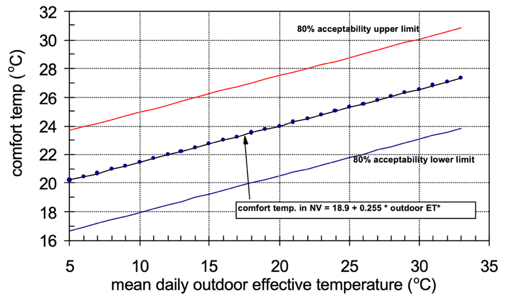
Figure 3.1: Comfort temperature in relation to outdoor temperature in non-cooled buildings with natural ventilation in RP-884. The red and blue lines indicate respectively the upper and lower limits of the range within which the thermal environment is acceptable for 80% of the occupants. Source: de Dear et al, 1997.

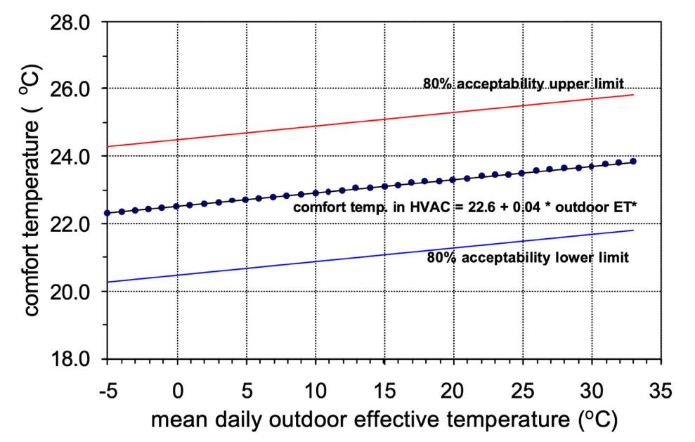
Figure 3.2: Comfort temperature in relation to outdoor temperature in buildings with central air conditioning in RP-884. The red and blue lines indicate respectively the upper and lower limits of the area within which the thermal environment is acceptable for 80% of the occupants. Source: de Dear et al, 1997.

Next, in RP-884, the relationship between the neutral temperature and the mean effective outdoor temperature in the month in question is calculated. In the latest version of the ASHRAE standard, the mean outdoor temperature has been replaced by the prevailing8 outdoor temperature (ASHRAE 55, 2017). This results, for example, in the middle lines in Figure 3.1 and Figure 3.2. Finally, a bandwidth is shown around these lines, within which the thermal environment is acceptable for 80% of the occupants. Two assumptions are made here, namely that a vote on one of the three middle categories of the ASHRAE scale means the thermal environment is acceptable and that the distribution of votes on the ASHRAE scale within each building is sufficiently similar to the distribution of the PPD function in the PMV model to assume that a vote on the ASHRAE scale of +0.85 or -0.85 corresponds to 80% overall acceptability (20% dissatisfied). These are for example the lower and upper lines in Figure 3.1 and Figure 3.2. In the same way, limits for 90% acceptability can be calculated. These Figures show that:

Comfort temperatures are related to the mean outdoor temperature: the warmer it is outside, the higher the comfort temperature indoors. Building users get accustomed to and adapt to temperatures that vary along with the outside temperature;

The comfort temperature in naturally ventilated, uncooled buildings is more closely related to the outside temperature than in air-conditioned buildings.

3.3 European adaptive thermal comfort field study

A second major study was commissioned by the EU with the aim of reducing energy use in air-conditioned buildings and encouraging the use of naturally ventilated, free-running buildings through the development of control systems based on adaptive comfort. This so-called SCATs study consists of building surveys carried out several times over a year in 26 office buildings in France, Greece, Portugal, Sweden and the UK (McCartney, 2002; Nicol & Humphreys, 2005). On a number of points, this study makes different assumptions from RP-884. Firstly, no regression equations per building are used to determine the neutral temperature. Instead, the relationship between the TSV and the operative temperature is assumed to have a fixed regression coefficient, called the Griffiths constant, named after its creator. The higher this regression coefficient, the stronger the relationship between the neutral temperature and the TSV. This constant cannot be derived directly from the data because observed regression coefficients are lower than actual values due to confounding factors. These can be:

Measurement errors in determining the operative temperature: there will always be some degree of measurement error;

Errors in the equation used to calculate the operative temperature: the optimal index for the ambient temperature may be slightly different from the operative temperature;

Behavioural adaptation: when the indoor temperature varies over a wider range, occupants are more likely to adjust their clothing insulation, so the observed regression coefficient is lower than the actual value;

Psychological adaptation: occupants accustomed to a wider range of indoor temperatures may be less sensitive to changes in temperature than those accustomed to a narrower range, so that with a wider range of indoor temperatures the observed regression coefficient is lower than the actual value.

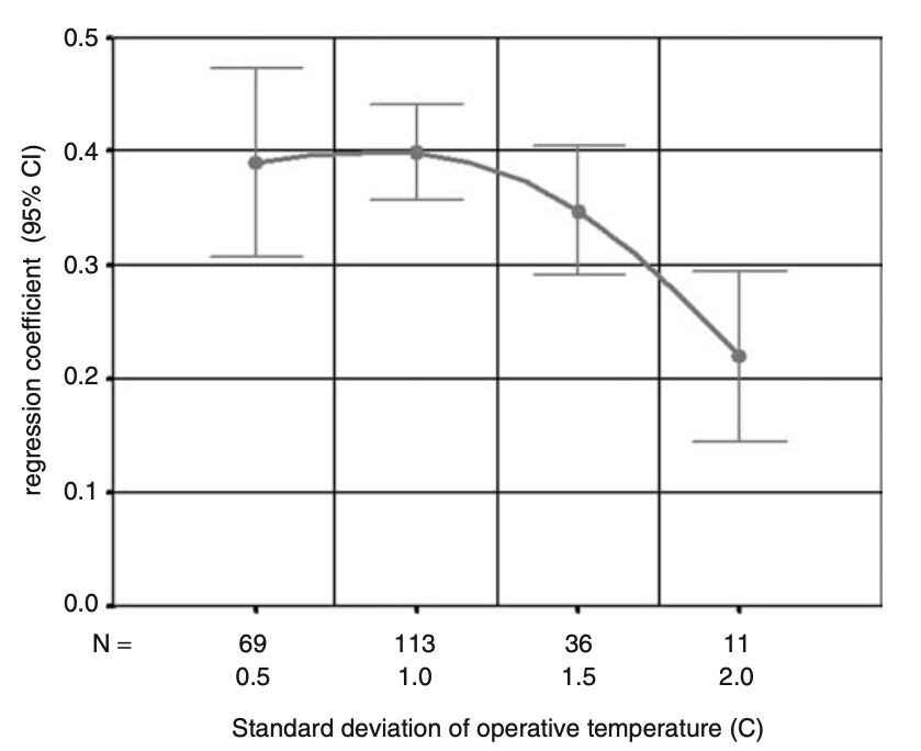
Figure 3.3: Mean values of regression coefficients and standard deviation of operative temperature in RP-884 and SCATs databases. Sources: Nicol & Humphreys, 2005.

Figure 3.3 shows the relationship between the observed regression coefficient and the standard deviation (statistical measure of scatter) of the indoor operative temperature. The curve shows a maximum of about 0.4 with a standard deviation of the indoor temperature of about 1.0. Below this, the regression coefficient is slightly lower, which is probably due to measurement errors and errors in the equation used, which count more heavily when the indoor temperature spread is low. Above that, the greater the distribution of indoor temperatures, the lower the regression coefficient, which is probably due to behavioural adaptation and possibly also psychological adaptation. As there is also likely to be some reduction in the observed regression coefficient of 0.4 due to confounding factors, a regression coefficient of 0.5 is chosen in the SCATs study. With this fixed regression coefficient, the neutral temperature can be calculated from any combination of a TSV and an operative temperature by the following equation:

Neutral temperature = operative temperature - TSV / 0.5 (1)

Next, the relationship between the neutral temperature and the outdoor temperature is determined. In RP-884, the mean of the daytime and night-time temperatures for the month in question is used. The SCATs study, on the other hand, uses the running mean outdoor temperature, RMOT, in the equation below: Trm. This is determined as follows:

Trm = (1- α) . (Tod-1 + α. Tod-2 + α2Tod-3 + α3Tod-4 + ...)

where:

Trm =running mean outdoor temperature;

Tod-1 = Mean of maximum and minimum outdoor temperature yesterday;

Tod-2 = Mean of maximum and minimum outdoor temperature day before yesterday;

Tod-3 = Mean of maximum and minimum outdoor temperature day before day before yesterday;

Tod-4 = etc.

α is a constant that defines the speed at which the running mean responds to the outside temperature. Usually, a value of 0.8 is used. This equation implies that the Mean comfort temperatures in buildings can be determined on the basis of an Mean outdoor temperature of the past few days, with the most recent days being weighted most strongly. The reason for this is that the SCATs study shows that the influence of the outdoor temperature on the expectations of the occupants and on the choice of the clothing is determined by the days immediately preceding the day in question, with the most recent days weighted the strongest. Finally, as in RP-884, a range is given within which the indoor temperature must fall to ensure that enough occupants feel comfortable. In RP-884 this was derived from the PPD equation in the PMV model, in the SCATs study it is done on the basis of an observed relationship between deviation of actual temperature from neutral temperature and the percentage of occupants who feel comfortable (Figure 6.1). This then leads to temperature limits as shown in Figure 6.2. The SCATs study distinguished between free running on the one hand and heated and cooled conditions on the other, which yielded different relationships (Figure 3.4).

Figure 3.4: Mean indoor comfort temperatures for free running (solid lines) and heated and cooled buildings (dashed line) depending on the running mean outdoor temperature (SCATs study). Source: Nicol & Humphreys, 2005.

Formally, the standards based on the RP-884 and the SCATs studies should not be compared because there are so many differences in the way they were developed. However, it is informative to do so for the following reasons. The locations where both surveys were conducted are largely different, but there is also overlap. Furthermore, the differentiation in climate between the locations in RP-884 should also make this study sufficiently representative for Europe. Calculating neutral temperatures per building based on the data for that building, as in RP-884, or deriving a constant regression coefficient from the total data, as in the SCATs study, are both legitimate methods. Establishing temperature limits based on the PPD equation in the PMV model, as in RP-884, or based on an observed relationship, as in the SCATs study, are also both legitimate methods. The only point where the difference in approach does matter is the measure of outdoor temperature, which is more appropriate in the SCATs study than in RP-884. When the bandwidths of RP-884 and SCATs are compared it becomes apparent that the difference is small, especially in the upper limits for 80% satisfaction. Both upper limits are almost parallel and have a difference in the allowable operative temperature of up to 1K. The great similarity between the standards based on RP-884 and the SCATs study, respectively, confirms the validity of the results of both studies and the standardisation based on them. The main reason for choosing the European standard based on the SCATs study is not only that this study is more representative for the European situation, but also because of the better measure of the outside temperature: the running mean outdoor temperature (RMOT).

In Figure 3.5, the neutral or comfort temperatures of each building studied are within a certain range. The distance to the mean regression line is not a measurement error, but are the actual comfort temperatures (Humphreys & Nicol, 2018). This means that different mean indoor comfort temperatures are found for each outdoor temperature and that there are therefore local differences in the relationship between outdoor and indoor comfort temperatures. Thus, in different climates and buildings there are different relationships between outdoor temperature and comfort temperature, but they are all within the range shown in Figure 3.5.

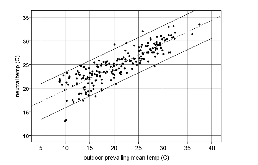
Figure 3.5: The relationship between the neutral temperature and the prevailing outdoor temperature based on the RP-884 and SCATs databases. Each point is a separate survey. Source: Nicol & Humphreys, 2005.

For example, the SCATs data provide the normative relationship for European buildings and similar climates and cultures, but this may differ from, for example, India (Manu et al., 2016) and southern Brazil (Rupp et al., 2018a). Furthermore, most research has been conducted in offices and little is known about thermal comfort and adaptive behaviour in homes, schools and healthcare facilities. It is therefore of great importance that such research is conducted in different climate zones and types of buildings to further perfect the adaptive model. A first initiative in this direction is described in Chapter 8.

Figure 3.6 compares the comfort temperatures predicted by the PMV model with the observed comfort temperatures for the naturally ventilated buildings. The PMV model is somewhat adaptive, as one can take into account the differences in clothing insulation over the seasons, so that at least part of the behavioural adaptation is taken into account. Therefore, there is a certain relationship between the outdoor temperature and the calculated neutral indoor temperature (the red line in Figure 3.6). However, in naturally ventilated (non-cooled) environments, the PMV model does not appear to predict thermal comfort well. For outdoor temperatures above 20°C it predicts a lower comfort temperature than is observed, which corresponds to the PMV model's overestimation of thermal comfort mentioned earlier (Figure 2.7). For outdoor temperatures below 20°C it predicts a higher comfort temperature than is observed (Figure 2.7). This is because in free running environments the temperature that people subconsciously expect is dependent on the temperatures of the past few days. As a result, in free running environments comfort temperatures are in fact more closely related to outside temperatures than the PMV model shows (de Dear & Brager, 2002), as illustrated by the blue line in Figure 3.6.

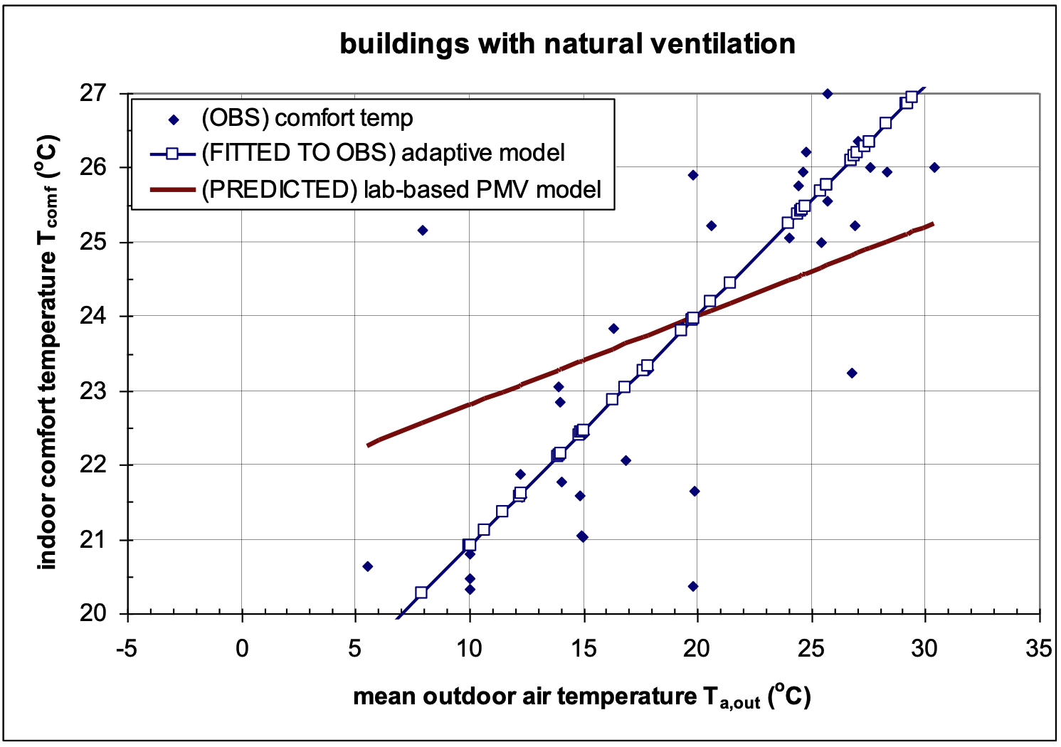
Figure 3.6: Comfort temperatures predicted by the PMV model (PREDICTED) compared to observed comfort temperatures (OBS) in naturally ventilated buildings and the calculated relationship between the observed comfort temperature and the Mean monthly outdoor temperature for naturally ventilated buildings (FITTED TO OBS). Source: Nicol & Humphreys, 2005.